
In this article we will see how to provision a redshift cluster, load some large quantity of data from s3 and run a query to see the contents and check performance. I plan to write a serie of articles arround data warehousing in the cloud so check out for new articles where i will do someting similar but from Synapse, Snowflake and Databricks Delta.
I’ve split the article in 4 steps that cover diverse topics:
- Part 1. Deploying a redshift cluster.
- Part 2. Load TPC-DS data.
- Part 3. Run queries to verify the performance.
- Part 4. Performance tricks.
- Deploying a redshift cluster
As always with cloud providers, we have many ways to deploy resources. We can use the native tools (aws cli) or the portal, or we can use some external software, like terraform.
For this example we will go through the aws portal as we only plan to create one for test purposes. If you never created one, there is a promotion on aws that let’s you to create a two month dc2.Large node for free.
To create the cluster go to the redshift area of the aws portal here and click on create cluster. For this we will need to define the name of the cluster, the size and the type of cluster (production, free test), the number of nodes, the name of the database, admin username and password, the port and other aspects like vpc and subnet, security groups, parameter group and backup policies we want to apply. We can leave the defaults for these. For the rest of values choose non used ones and a strong user and password combination. If you want to use the free ofer, make sure you select the same as me:
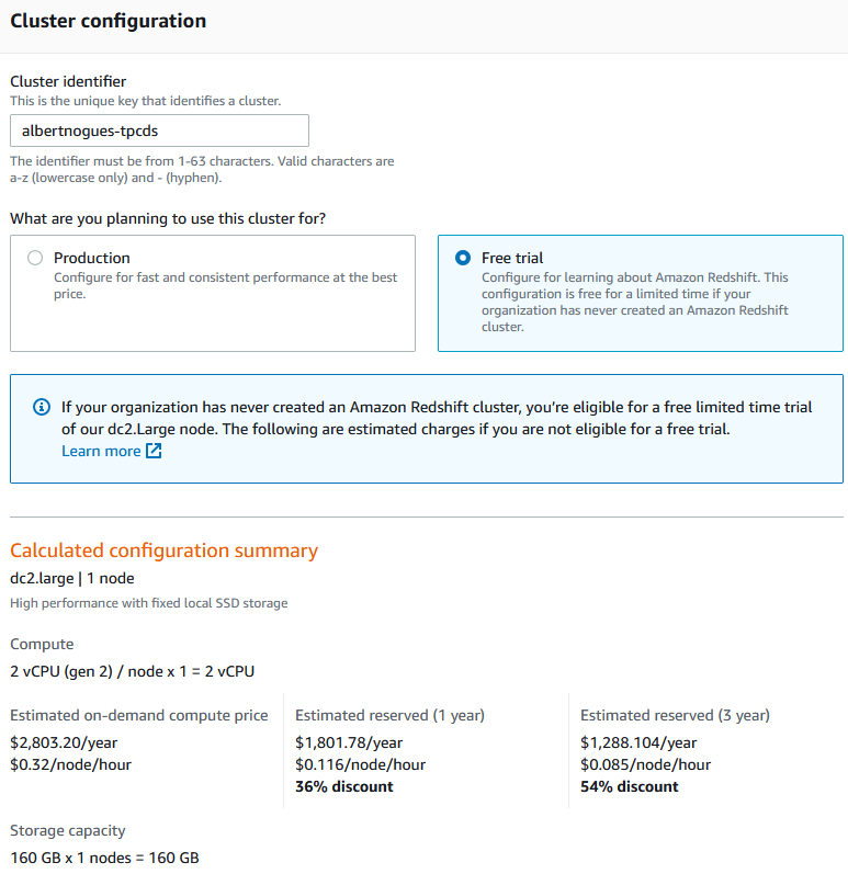
The fill the rest of the information and press the create cluster button. In a few minutes the cluster will be up and running.
2. Load TPC-DS Data
Before starting loading the data, let’s connect to our brand new cluster. For connecting, we can use the integrated editor in the aws portal or use some other software like dbeaver. I personally recommend the latter as it’s more flexible. If our usual client does not support redshift we can always use the postgre driver.
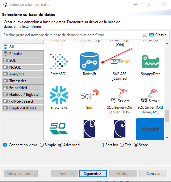
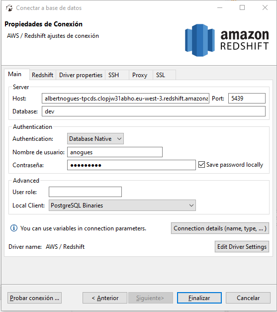
Then, DBeaver will automatically download the jar driver from internet unless we already have it and we then have to configure our connection:
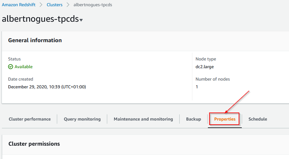
But before connecting, lets open the port in the security group. For this we need to go to our cluster in the aws portal, click on properties:
And check for the Network and Security section. If we want to access the cluster from our computer, as it’s the case (although in a corporate environment probably you dont want this!) we need to enable the publickly accessible section. This change will take some time.
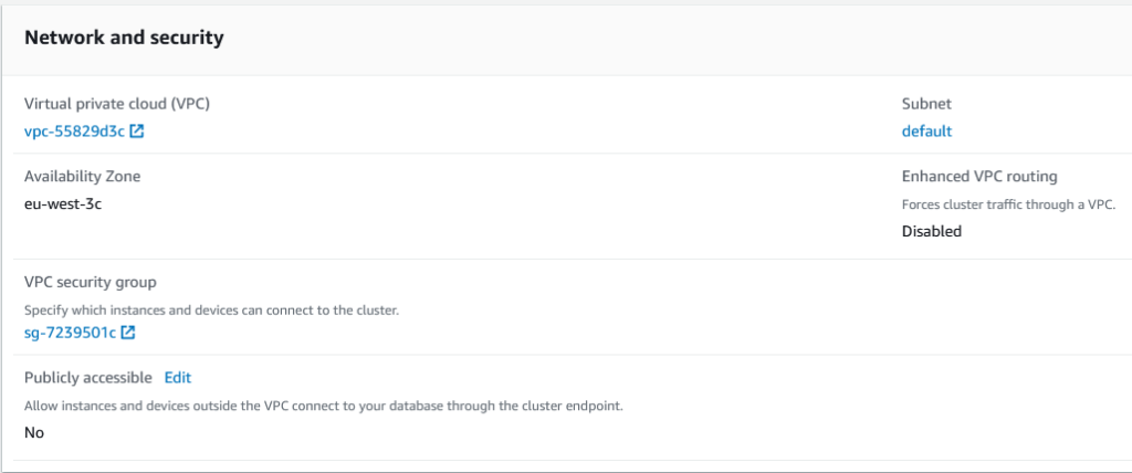
But before being able to connect we still have to click in the VPC security group and add a rule to be able to access redshift port from our location:
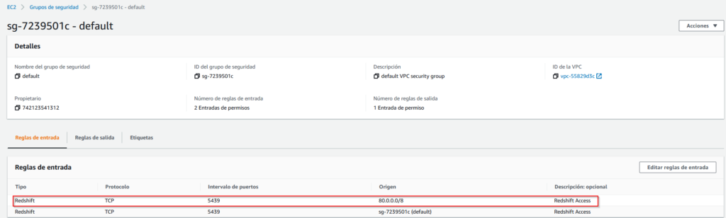
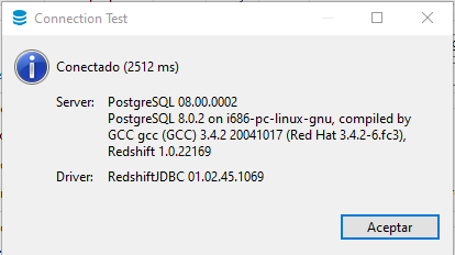
With this we can now test the connection from DBeaver, and now the connection should be succesful:
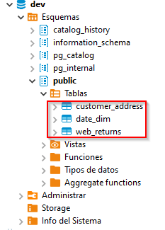
So, now, the next step is to load the information into redshift. For this, we will load some tables from a public s3 bucket maintained by aws. We will create four tables and then populate them from data in a public s3 bucket. We can get the ddl from here. We will crate the following three tables:
create table customer_address
(
 ca_address_sk int4 not null ,
  ca_address_id char(16) not null ,
  ca_street_number char(10) ,
  ca_street_name varchar(60) ,
  ca_street_type char(15) ,
  ca_suite_number char(10) ,
  ca_city varchar(60) ,
  ca_county varchar(30) ,
  ca_state char(2) ,
  ca_zip char(10) ,
  ca_country varchar(20) ,
  ca_gmt_offset numeric(5,2) ,
  ca_location_type char(20)
  ,primary key (ca_address_sk)
) distkey(ca_address_sk);

create table customer
(
  c_customer_sk int4 not null ,
  c_customer_id char(16) not null ,
  c_current_cdemo_sk int4 ,
  c_current_hdemo_sk int4 ,
  c_current_addr_sk int4 ,
  c_first_shipto_date_sk int4 ,
  c_first_sales_date_sk int4 ,
  c_salutation char(10) ,
  c_first_name char(20) ,
  c_last_name char(30) ,
  c_preferred_cust_flag char(1) ,
  c_birth_day int4 ,
  c_birth_month int4 ,
  c_birth_year int4 ,
  c_birth_country varchar(20) ,
  c_login char(13) ,
  c_email_address char(50) ,
  c_last_review_date_sk int4 ,
  primary key (c_customer_sk)
) distkey(c_customer_sk);

create table date_dim
(
    d_date_sk                 integer               not null,
    d_date_id                 char(16)              not null,
    d_date                    date,
    d_month_seq               integer                       ,
    d_week_seq                integer                       ,
    d_quarter_seq             integer                       ,
    d_year                    integer                       ,
    d_dow                     integer                       ,
    d_moy                     integer                       ,
    d_dom                     integer                       ,
    d_qoy                     integer                       ,
    d_fy_year                 integer                       ,
    d_fy_quarter_seq          integer                       ,
    d_fy_week_seq             integer                       ,
    d_day_name                char(9)                       ,
    d_quarter_name            char(6)                       ,
    d_holiday                 char(1)                       ,
    d_weekend                 char(1)                       ,
    d_following_holiday       char(1)                       ,
    d_first_dom               integer                       ,
    d_last_dom                integer                       ,
    d_same_day_ly             integer                       ,
    d_same_day_lq             integer                       ,
    d_current_day             char(1)                       ,
    d_current_week            char(1)                       ,
    d_current_month           char(1)                       ,
    d_current_quarter         char(1)                       ,
    d_current_year            char(1)                       ,
    primary key (d_date_sk)
) diststyle all;

create table web_returns
(
wr_returned_date_sk int4 ,
  wr_returned_time_sk int4 ,
  wr_item_sk int4 not null ,
  wr_refunded_customer_sk int4 ,
  wr_refunded_cdemo_sk int4 ,
  wr_refunded_hdemo_sk int4 ,
  wr_refunded_addr_sk int4 ,
  wr_returning_customer_sk int4 ,
  wr_returning_cdemo_sk int4 ,
  wr_returning_hdemo_sk int4 ,
  wr_returning_addr_sk int4 ,
  wr_web_page_sk int4 ,
  wr_reason_sk int4 ,
  wr_order_number int8 not null,
  wr_return_quantity int4 ,
  wr_return_amt numeric(7,2) ,
  wr_return_tax numeric(7,2) ,
  wr_return_amt_inc_tax numeric(7,2) ,
  wr_fee numeric(7,2) ,
  wr_return_ship_cost numeric(7,2) ,
  wr_refunded_cash numeric(7,2) ,
  wr_reversed_charge numeric(7,2) ,
  wr_account_credit numeric(7,2) ,
  wr_net_loss numeric(7,2)
  ,primary key (wr_item_sk, wr_order_number)
) distkey(wr_order_number) sortkey(wr_returned_date_sk);
You can create a new schema or use the public one for this test. I’ve created all four in the public schema.
Once the tables have been created, then lets populate them. To populate the four tables we need to pass some AWSKeys or a Role with permission to read data from S3 (even if the bucket is public). If it’s a one off job maybe the keys can be quick to set up, but if we intend to do this often, we should create an IAM role and attach it to the Redshift cluster. We will go this second way. For this lets go to the IAM portal and create a new role following this instructions.
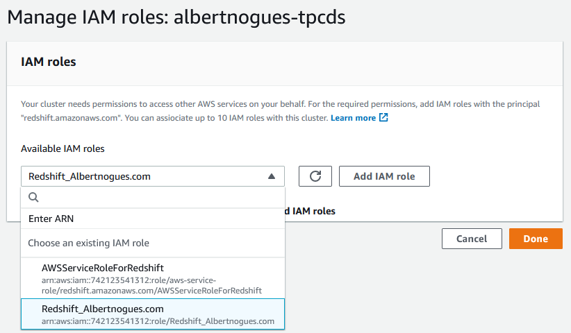
Then in the Redshift section, go to Actions, Manage IAM Roles, find your new IAM role and add it to the redshift cluster
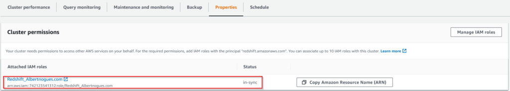
After a few seconds / minutes you should see the new role being added to the cluster:
Then we are ready to move to DBeaver and start the data loading. Since we have to load three tables we will use the following commands (First click on copy Amazon Resource Name (ARN) from the role we just added to our cluster, and then ran the three following commands (leave the region as us-east-1 no matter from where you are launching it as the data we are loading it’s in a bucket in that region. And replace my ARN by yours:
copy customer_address from 's3://redshift-downloads/TPC-DS/2.13/3TB/customer_address/' credentials 'aws_iam_role=arn:aws:iam::742123541312:role/Redshift_Albertnogues.com' gzip delimiter '|' EMPTYASNULL region 'us-east-1';

copy customer from 's3://redshift-downloads/TPC-DS/2.13/3TB/customer/' credentials 'aws_iam_role=arn:aws:iam::742123541312:role/Redshift_Albertnogues.com' gzip delimiter '|' EMPTYASNULL region 'us-east-1';

copy date_dim from 's3://redshift-downloads/TPC-DS/2.13/3TB/date_dim/' credentials 'aws_iam_role=arn:aws:iam::742123541312:role/Redshift_Albertnogues.com' gzip delimiter '|' EMPTYASNULL region 'us-east-1';

copy web_returns from 's3://redshift-downloads/TPC-DS/2.13/3TB/web_returns/' credentials 'aws_iam_role=arn:aws:iam::742123541312:role/Redshift_Albertnogues.com' gzip delimiter '|' EMPTYASNULL region 'us-east-1';
The load of the data should finish sucesfully after several minutes. For the biggest table (web_returns) it took me 50 minutes. After the load we can do a few checks (counts):
select 'customer_address' table_name, count (*) from customer_address
UNION
select 'customer' table_name, count (*) from customer
UNION
select 'date_dim' table_name, count (*) from date_dim
UNION
select 'web_returns' table_name, count (*) from web_returns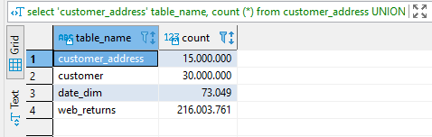
select count(*) from customer_address;  -- 15000000
select count(*) from customer;  -- 30000000
select count(*) from date_dim;  -- 73049
select count(*) from web_returns;  -- 216003761
3. Query the data
We can now launch a query to see the results:
-- start template query30.tpl query 3 in stream 1
with /* TPC-DS query30.tpl 0.75 */ customer_total_return as
 (select wr_returning_customer_sk as ctr_customer_sk
        ,ca_state as ctr_state,
 	sum(wr_return_amt) as ctr_total_return
 from web_returns
     ,date_dim
     ,customer_address
 where wr_returned_date_sk = d_date_sk
   and d_year =2002
   and wr_returning_addr_sk = ca_address_sk
 group by wr_returning_customer_sk
         ,ca_state)
  select  c_customer_id,c_salutation,c_first_name,c_last_name,c_preferred_cust_flag
       ,c_birth_day,c_birth_month,c_birth_year,c_birth_country,c_login,c_email_address
       ,c_last_review_date_sk,ctr_total_return
 from customer_total_return ctr1
     ,customer_address
     ,customer
 where ctr1.ctr_total_return > (select avg(ctr_total_return)*1.2
 			  from customer_total_return ctr2
                  	  where ctr1.ctr_state = ctr2.ctr_state)
       and ca_address_sk = c_current_addr_sk
       and ca_state = 'OH'
       and ctr1.ctr_customer_sk = c_customer_sk
 order by c_customer_id,c_salutation,c_first_name,c_last_name,c_preferred_cust_flag
                  ,c_birth_day,c_birth_month,c_birth_year,c_birth_country,c_login,c_email_address
                  ,c_last_review_date_sk,ctr_total_return
limit 100;
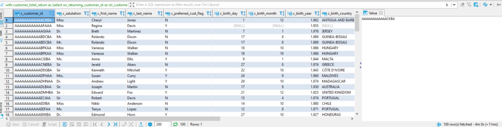
And the query returns the first 100 results in just 4 minutes:
4. Performance Tricks
With Redshift as almost all databases, there is always room for improvement. The possibilities for tuning start with compression and then go to distribution and sort keys. Right now, after loading the 4 tables, these are taking (we can see in storage used in the main page of our cluster in the aws redshift portal) :
11.88% (19.01 of 160 GB used)
Which is not bad taking into account that in .gz the size of the files in total is about 15.37 GB, so the db has done pretty much a good job (Caution, while loading you need much more space than this, as the bulk load needs stagging space before being able to optimize it, based on my tests you need 3 times the final space at least) . But this can be improved. We didnt specify any compression when we defined our table structure. The rationale here is that if we compress the data, the engine wil process less volume of data and the resoults should come faster right?. Let’s see:
analyze compression customer;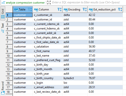
As we can see there are optimizations to be made to save both space (and possibly) processing time. Let’s create a better table:
create table customer_compressed
(
  c_customer_sk int4 encode delta not null ,
  c_customer_id char(16) encode zstd not null ,
  c_current_cdemo_sk int4 encode az64,
  c_current_hdemo_sk int4 encode az64,
  c_current_addr_sk int4 encode az64,
  c_first_shipto_date_sk int4 encode az64,
  c_first_sales_date_sk int4 encode az64  ,
  c_salutation char(10) encode zstd,
  c_first_name char(20) encode zstd,
  c_last_name char(30) encode zstd,
  c_preferred_cust_flag char(1)  encode zstd,
  c_birth_day int4 encode az64,
  c_birth_month int4 encode az64,
  c_birth_year int4 encode az64,
  c_birth_country varchar(20) encode bytedict,
  c_login char(13) encode lzo,
  c_email_address char(50) encode zstd,
  c_last_review_date_sk int4 encode az64,
  primary key (c_customer_sk)
) distkey(c_customer_sk);
And then insert back:
insert into customer_compressed select * from customer;And then later:
SELECT "table", tbl_rows, size size_in_MB FROM SVV_TABLE_INFO
order by 1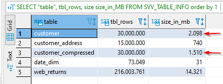
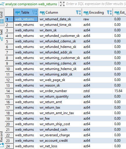
So we easily saved 25% of space in this table. Let’s do the same for the rest (mainly for web_returns, the others are small so probably no need to compress them)
analyze compression web_returns;but unfortunately we see that there is no improvement to be made.
So the compression is over. Next steps are the distribution and the sort keys but being tpc-ds queries these have been already optimized for the tpc-ds queries. For this you can follow the excellent guide in aws documentation here.